Diagnostic plots based on one-step-ahead residuals

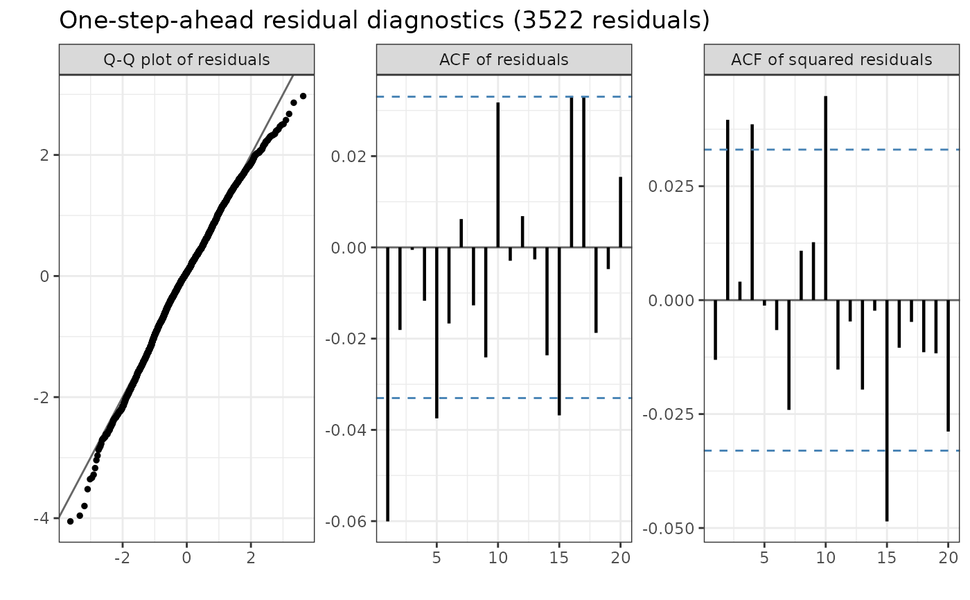
Shows three panels that check if the fitted model describes the data:

• A Q-Q plot of the one-step-ahead (OSA) residuals against the standard gaussian distribution. If the model is correct, the points follow the diagonal. Bent tails show that the error distribution is wrong, for example that the returns have heavier tails or more skewness than the model allows.

• The autocorrelation function (ACF) of the residuals. Bars outside the dashed lines show dependence in the returns that the model does not capture.

• The ACF of the squared residuals. Bars outside the dashed lines show volatility clustering that the model does not capture.

Usage

plot_diagnostics(x, res = NULL, lag_max = 20, ...)

Arguments

x

A stochvolTMB object returned from estimate_parameters.

res

Optional vector of OSA residuals from residuals. If NULL, the residuals are calculated.

lag_max

Maximum lag in the ACF panels.

...

Arguments passed to residuals when res is NULL, for example method or conditional.

Value

ggplot object with the three diagnostic panels.

Details

By default, the residuals are calculated for all observations with the exact grid method of residuals, which takes a few seconds. To reuse residuals, calculate them once with residuals and give them in res.

Examples

# \donttest{
data(spy)
opt <- estimate_parameters(spy$log_return, model = "t", silent = TRUE)
plot_diagnostics(opt)

# }