stochvolTMB: Likelihood estimation of stochastic volatility

Jens Christian Wahl

The stochastic volatility model

The stochastic volatility model, introduced by Taylor (1982), is defined by \[\begin{equation} \begin{aligned} y_t &= \sigma_y e^{h_t/2} \epsilon_t, \quad t = 1, \dots, T, \\ h_{t+1} &= \phi h_{t} + \sigma_h \eta_t, \quad t = 1, \dots, T-1, \\ \eta_t &\stackrel{\text{iid}}{\sim} \mathcal{N}(0,1), \\ \epsilon_t &\stackrel{\text{iid}} {\sim} F \end{aligned} \end{equation}\] where \(y_t\) is the observed log returns, \(h_t\) is the logarithm of the variance on day \(t\). The distribution of the innovations \(\epsilon_t\) is specified below. To ensure stationarity for \(h_t\), we assume \(|\phi| < 1\). It can be shown that the unconditional distribution of \(h_t\) is \(\mathcal{N}(0,\sigma_h^2/(1 - \phi^2))\), and we assume \(h_1 \sim \mathcal{N}(0,\sigma_h^2/(1-\phi^2))\). An interpretation of the latent process \(\{h_t\}\) is that is represents the random and uneven flow of new information into the marked. For different time points, the variance will be dependent of this unobserved ``flow’’ of information, i.e. conditioning on \(h_t\), \(\mathrm{Var}(y_t | h_t) = \sigma_y^2 e^{h_t}\).

The original SV model from Taylor (1982) assumed normally distributed innovations, but this is usually to strong of an assumption. Financial returns are usually heavy-tailed, might be asymmetric and the volatility can be correlated with the returns. The latter is called the leverage effect, where there is a negative correlation between a change in price and the volatility, meaning that a drop in price tend to lead to an increase in volatility To take these features of financial time series into account stochvolTMB has implemented the following seven models for the innovations:

• Gaussian: \(\epsilon_t \sim \mathcal{N}(0,1)\)
• t: \(\epsilon_t \sim t_\nu(0,1)\), where \(\nu\) is the degrees of freedom.
• Skew-Gaussian: \(\epsilon_t \sim \mathcal{SN}(0,1, \alpha)\), with zero mean, unit variance and shape parameter \(\alpha\). See Skewness and the shape parameter for how the asymmetry is estimated and reported.
• Leverage: \(\epsilon_t \sim \mathcal{N}(0,1)\) and \(\mathrm{Cor}(\epsilon_t, \eta_t) = \rho\)
• Skew-Gaussian with leverage: \(\epsilon_t \sim \mathcal{SN}(0,1, \alpha)\) and \(\eta_t = \rho \epsilon_t + \sqrt{1 - \rho^2} e_t\), where \(e_t \sim \mathcal{N}(0,1)\) is independent of \(\epsilon_t\). Then \(\mathrm{Cor}(\epsilon_t, \eta_t) = \rho\), and the returns have the same skewness as in the skew-Gaussian model. With \(\alpha = 0\) this is the leverage model.
• Skew-t: \(\epsilon_t\) has the skew t distribution of Jones and Faddy (2003), scaled to zero mean and unit variance. Its density is proportional to \((1 + x/\sqrt{a + b + x^2})^{a + 1/2} (1 - x/\sqrt{a + b + x^2})^{b + 1/2}\) before scaling. The left tail decays like a t-distribution with \(\nu_L = 2a\) degrees of freedom, and the right tail like one with \(\nu_R = 2b\). With \(\nu_L < \nu_R\), large losses are more likely than large gains, which is common for stock returns. With \(\nu_L = \nu_R\) this is the t model.
• Skew-t with leverage: \(\epsilon_t\) has the skew t distribution above, and \(\eta_t = \rho \epsilon_t + \sqrt{1 - \rho^2} e_t\) as in the skew-Gaussian model with leverage. This combines heavy and asymmetric tails with the leverage effect.

Skewness and the shape parameter

The skew-Gaussian models report two numbers for the asymmetry of \(\epsilon_t\): the shape parameter alpha and the skewness. Both describe the same distribution on different scales.

The shape parameter \(\alpha\) is the parameter of the skew-normal density. With location \(\xi\) and scale \(\omega\) chosen so that \(\epsilon_t\) has mean zero and unit variance, the density is \[ p(x) = \frac{2}{\omega} \phi\left(\frac{x - \xi}{\omega}\right) \Phi\left(\alpha \frac{x - \xi}{\omega}\right), \] where \(\phi\) and \(\Phi\) are the density and the distribution function of the standard Gaussian distribution. \(\alpha = 0\) gives the Gaussian distribution, and \(\alpha \to \pm \infty\) gives a half-Gaussian distribution. \(\alpha\) has no direct statistical meaning.

The skewness \(\gamma_1 = \mathrm{E}[\epsilon_t^3]\) is the usual skewness coefficient, because \(\epsilon_t\) has mean zero and unit variance. It is a monotone function of \(\alpha\): \[ \delta = \frac{\alpha}{\sqrt{1 + \alpha^2}}, \qquad \mu = \delta \sqrt{2 / \pi}, \qquad \gamma_1 = \frac{4 - \pi}{2} \frac{\mu^3}{(1 - \mu^2)^{3/2}}. \]

\(\alpha\)	0	0.5	1	2	5	27	\(\infty\)
\(\gamma_1\)	0	0.02	0.14	0.45	0.85	0.99	0.995

stochvolTMB estimates the skewness, not \(\alpha\), for two reasons:

• Close to zero, \(\gamma_1\) grows like \(\alpha^3\). The likelihood is therefore flat in \(\alpha\) at \(\alpha = 0\) (the first and second derivatives are zero), and an optimizer that starts there does not move. In the skewness, the likelihood has a normal slope at zero.
• Large values of \(\alpha\) change the distribution very little. The skewness is bounded by \(|\gamma_1| < 0.99\), which corresponds to \(|\alpha| \le 27\). This keeps the optimizer away from the half-Gaussian limit, where the fit is unstable.

The skewness is estimated on a transformed scale as logit_skewness. summary(object, report = "transformed") reports skewness and alpha with standard errors from the delta method. Use skewness for inference. Use alpha when you need the shape parameter, for example in sim_sv, sn::dsn or other software. When the skewness is close to zero, a small change in skewness gives a large change in \(\alpha\), so the standard error of alpha is very large even when the skewness is well determined.

In the skew-Gaussian model with leverage, the skewness is that of the return shock \(\epsilon_t\), not of the returns \(y_t\). The time-varying volatility, and its correlation with past shocks, change the distribution of \(y_t\).

stochvolTMB is inspired by the package stochvol (Kastner (2016)), but stochvolTMB obtain parameter estimates through maximum likelihood estimation and not Markov Chain Monte Carlo.

Usage

The main functions of stochvolTMB are:

Function Name	Description
estimate_parameters	Estimate parameters of a stochastic volatility model.
sim_sv	Simulate data from a stochastic volatility model.
plot.stochvolTMB	Plot estimated volatility and predicted (with confidence intervals).
summary.stochvolTMB	Extract parameter estimates and volatility with uncertainty.
predict.stochvolTMB	Predict future volatility and returns.
plot_returns	Plot returns with intervals from the fitted model.
residuals	Calculate one-step-ahead residuals.
plot_diagnostics	Plot diagnostics based on one-step-ahead residuals.
compare_models	Fit several models and rank them by AIC.
coef, vcov	Parameter estimates and their covariance matrix.
var_es	One-day Value at Risk and Expected Shortfall.
forecast_var_es	Value at Risk and Expected Shortfall for several days.
backtest_var	Backtest the Value at Risk.
plot_var	Plot returns with the Value at Risk and Expected Shortfall.

estimate_parameters returns an object of class stochvolTMB. The summary function returns a data.table with estimated parameters, estimated log-volatility and transformed parameters along with standard errors, p-values and z-values. The argument report = "fixed" returns the parameters on the scale they were estimated. This means that the standard deviations \(\sigma_y, \sigma_h\) are given on the log scale; the degrees of freedom is one the scale \(\log (\nu - 2)\) to ensure that \(\nu > 2\) (i.e. the variance exists); and lastly that the persistence parameter \(\phi\) and the correlation parameter \(\rho\) are estimated on a logit scale to ensure that they are between -1 and 1. If report = c("fixed", "transformed"), parameter estimates transformed back to their original scale is also returned. If you want to extract the estimated log-volatility you can use report = "random".

Example

Estimating parameters in a SV model is easy with stochvolTMB. As an example we investigate the daily log-returns of the S&P500 from 2005 to 2018. A quick look at the data:

data(spy)
plot(spy$date, spy$log_return, type = "l", xlab = "", ylab = "", main = "Log-returns of S&P500")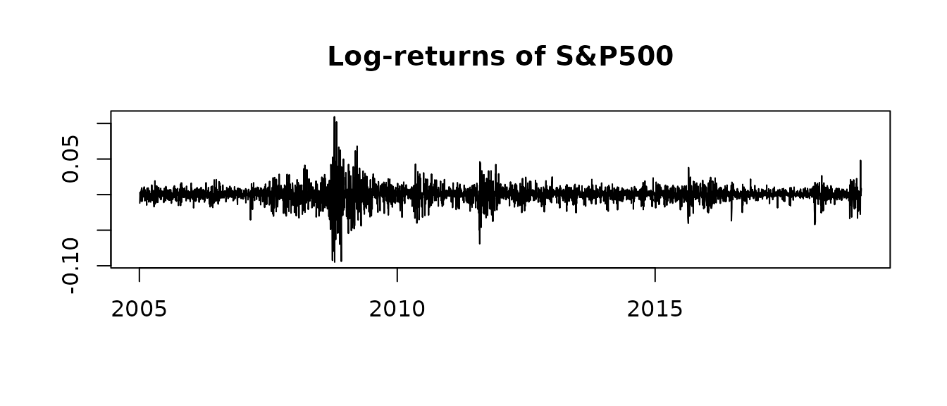

plot(spy$date, spy$price, type = "l", xlab = "", ylab = "", main = "Price of S&P500")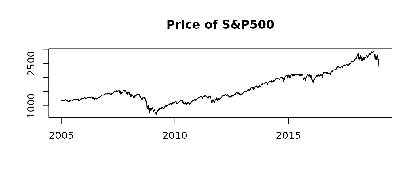

We fit all seven models with compare_models. It calls estimate_parameters for each model and stores the fitted models in the attribute "fits". To fit one model, use estimate_parameters(spy$log_return, model = "leverage").

comparison <- compare_models(spy$log_return)
fits <- attr(comparison, "fits")
gaussian <- fits$gaussian
t_dist <- fits$t
skew_gaussian <- fits$skew_gaussian
leverage <- fits$leverage
skew_gaussian_leverage <- fits$skew_gaussian_leverage
skew_t <- fits$skew_t
skew_t_leverage <- fits$skew_t_leverage

We can investigate the estimate for the degrees of freedom (df) to see if the returns are heavy-tailed

summary(t_dist, report = "transformed")
#>    parameter     estimate    std_error    z_value      p_value        type
#>       <char>        <num>        <num>      <num>        <num>      <char>
#> 1:   sigma_y  0.008392879 0.0008689248   9.658924 4.505714e-22 transformed
#> 2:   sigma_h  0.185766767 0.0182175649  10.197124 2.042308e-24 transformed
#> 3:       phi  0.984924644 0.0039281816 250.732972 0.000000e+00 transformed
#> 4:        df 10.086366735 2.1022435029   4.797906 1.603330e-06 transformed

Clearly the returns are more heavy tailed than Gaussian, even when controlling for the stochastic volatility. We can also check for asymmetric returns

summary(skew_gaussian, report = "transformed")
#>    parameter     estimate    std_error    z_value      p_value        type
#>       <char>        <num>        <num>      <num>        <num>      <char>
#> 1:   sigma_y  0.008247888 0.0007528397  10.955703 6.239189e-28 transformed
#> 2:   sigma_h  0.210904249 0.0187693205  11.236648 2.694187e-29 transformed
#> 3:       phi  0.980555386 0.0044991195 217.943839 0.000000e+00 transformed
#> 4:  skewness -0.164420269 0.0452041263  -3.637285 2.755275e-04 transformed
#> 5:     alpha -1.088785163 0.1427623077  -7.626559 2.411026e-14 transformed

and leverage (rho)

summary(leverage, report = "transformed")
#>    parameter     estimate    std_error   z_value       p_value        type
#>       <char>        <num>        <num>     <num>         <num>      <char>
#> 1:   sigma_y  0.008338412 0.0004163314  20.02830  3.121144e-89 transformed
#> 2:   sigma_h  0.273443559 0.0182641070  14.97164  1.125191e-50 transformed
#> 3:       phi  0.967721215 0.0043681868 221.53842  0.000000e+00 transformed
#> 4:       rho -0.748695259 0.0322487815 -23.21623 3.121690e-119 transformed

There is clear evidence for both asymmetric returns and a negative correlation (of -0.74!) between log-returns and the volatility.

We can also check if combining skewness and leverage provides a better fit:

summary(skew_gaussian_leverage, report = "transformed")
#>    parameter     estimate    std_error   z_value       p_value        type
#>       <char>        <num>        <num>     <num>         <num>      <char>
#> 1:   sigma_y  0.007951179 0.0003805306  20.89498  5.948133e-97 transformed
#> 2:   sigma_h  0.276811702 0.0178393398  15.51693  2.665194e-54 transformed
#> 3:       phi  0.971016377 0.0038900968 249.61239  0.000000e+00 transformed
#> 4:  skewness -0.404691018 0.0391237332 -10.34388  4.461237e-25 transformed
#> 5:     alpha -1.829728834 0.1306960204 -13.99988  1.561303e-44 transformed
#> 6:       rho -0.837199898 0.0226025004 -37.04015 2.587850e-300 transformed

To find the model that fits the data best, we can compare the AIC of our models and pick the smallest. compare_models returns the models ranked by AIC. The columns converged and pd_hessian show if the optimizer converged and if the Hessian is positive definite. If one of them is FALSE, the estimates of that model are not reliable.

comparison[, .(model, n_par, log_lik, aic, bic, delta_aic, converged, pd_hessian)]
#>                     model n_par  log_lik       aic       bic delta_aic
#>                    <char> <int>    <num>     <num>     <num>     <num>
#> 1:        skew_t_leverage     6 11866.69 -23721.38 -23684.38   0.00000
#> 2: skew_gaussian_leverage     5 11854.30 -23698.59 -23667.76  22.78558
#> 3:               leverage     4 11808.43 -23608.85 -23584.18 112.52674
#> 4:                 skew_t     5 11734.86 -23459.72 -23428.89 261.65871
#> 5:                      t     4 11729.85 -23451.69 -23427.02 269.68665
#> 6:          skew_gaussian     4 11724.36 -23440.72 -23416.06 280.65545
#> 7:               gaussian     3 11718.29 -23430.57 -23412.07 290.80456
#>    converged pd_hessian
#>       <lgcl>     <lgcl>
#> 1:      TRUE       TRUE
#> 2:      TRUE       TRUE
#> 3:      TRUE       TRUE
#> 4:      TRUE       TRUE
#> 5:      TRUE       TRUE
#> 6:      TRUE       TRUE
#> 7:      TRUE       TRUE

The skew-t model with leverage has the smallest AIC. It estimates one degree of freedom for each tail and the leverage \(\rho\). The left tail of the S&P 500 returns is clearly heavier than the right tail, and the correlation between the return shock and the volatility shock is strongly negative:

summary(skew_t_leverage, report = "transformed")
#>    parameter     estimate    std_error    z_value      p_value        type
#>       <char>        <num>        <num>      <num>        <num>      <char>
#> 1:   sigma_y  0.007960947 0.0003943647  20.186762 1.279816e-90 transformed
#> 2:   sigma_h  0.266050222 0.0179234179  14.843721 7.639759e-50 transformed
#> 3:       phi  0.975054403 0.0035924730 271.415928 0.000000e+00 transformed
#> 4:   df_left  8.633937520 1.5493994858   5.572441 2.511943e-08 transformed
#> 5:  df_right 15.174233109 3.7766661081   4.017891 5.872132e-05 transformed
#> 6:       rho -0.870746610 0.0201355160 -43.244316 0.000000e+00 transformed

coef and vcov return the estimates on their natural scale and their covariance matrix. With scale = "estimation" they use the scale that the parameters were estimated on:

coef(skew_t_leverage)
#>      sigma_y      sigma_h          phi      df_left     df_right          rho 
#>  0.007960947  0.266050222  0.975054403  8.633937520 15.174233109 -0.870746610
sqrt(diag(vcov(skew_t_leverage)))
#>      sigma_y      sigma_h          phi      df_left     df_right          rho 
#> 0.0003943647 0.0179234179 0.0035924730 1.5493994858 3.7766661081 0.0201355160

We can compare the leverage model with the skew-Gaussian leverage model to see if adding skewness improves the fit.

The skew-Gaussian models report both skewness and the shape parameter alpha (see Skewness and the shape parameter). Use skewness for inference. To simulate from the model, give alpha to sim_sv:

param <- list(phi = 0.95, sigma_h = 0.25, sigma_y = 0.01, alpha = -2, rho = -0.7)
sim <- sim_sv(param, nobs = 2000, seed = 1, model = "skew_gaussian_leverage")
fit <- estimate_parameters(sim$y, model = "skew_gaussian_leverage", silent = TRUE)
summary(fit, report = "transformed")
#>    parameter    estimate    std_error    z_value       p_value        type
#>       <char>       <num>        <num>      <num>         <num>      <char>
#> 1:   sigma_y  0.01032339 0.0003779025  27.317593 2.621788e-164 transformed
#> 2:   sigma_h  0.23428648 0.0242279178   9.670104  4.039680e-22 transformed
#> 3:       phi  0.93945634 0.0113655485  82.658249  0.000000e+00 transformed
#> 4:  skewness -0.49637925 0.0541021455  -9.174853  4.521897e-20 transformed
#> 5:     alpha -2.15955500 0.2114230932 -10.214376  1.709754e-24 transformed
#> 6:       rho -0.70745466 0.0576766544 -12.265875  1.381115e-34 transformed

Lastly, we can also plot the estimated log-volatility and volatility:

plot(leverage, include_ci = TRUE, plot_log = TRUE, dates = spy$date)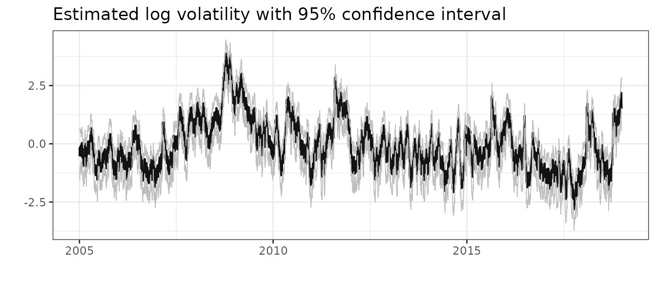

plot(leverage, include_ci = TRUE, plot_log = FALSE, dates = spy$date)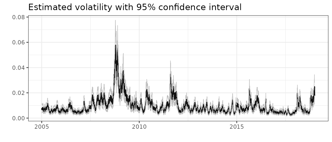

We can simulate future returns with predict. This function returns three matrices of dimension \(\#\) steps \(\times\) #$ simulations: (1) the latent log-volatility h; (2) one for the percentage volatility 100 * sigma_y * exp(0.5 * h) and (3) future returns. If the argument include_parameters is set to TRUE, the fixed parameters are simulated from their asymptotic multivariate distribution. This usually leads to broader uncertainty bands. To summarize the output from predict, we use the summary function, that calculate the mean and different quantiles based on the sumulations. We use the leverage model as an example:

pred = predict(leverage, steps = 10, include_parameters = TRUE)
summary(pred)
#> $y
#>      time quantile_0.025 quantile_0.975          mean
#>     <int>          <num>          <num>         <num>
#>  1:     1    -0.03390928     0.03578714  1.884305e-04
#>  2:     2    -0.03468329     0.03533891  1.936343e-04
#>  3:     3    -0.03399761     0.03578401  5.544499e-04
#>  4:     4    -0.03539847     0.03482133 -7.306338e-05
#>  5:     5    -0.03507907     0.03531515 -1.994870e-04
#>  6:     6    -0.03346930     0.03283918  3.510375e-05
#>  7:     7    -0.03382748     0.03325664 -6.717707e-05
#>  8:     8    -0.03510687     0.03489823  5.258260e-05
#>  9:     9    -0.03276020     0.03321078 -5.889527e-05
#> 10:    10    -0.03267239     0.03235914  7.830765e-05
#> 
#> $h
#>      time quantile_0.025 quantile_0.975     mean
#>     <int>          <num>          <num>    <num>
#>  1:     1     0.31931862       2.334532 1.339585
#>  2:     2     0.17822570       2.395486 1.292486
#>  3:     3     0.02750050       2.430255 1.248190
#>  4:     4    -0.09583098       2.470918 1.200189
#>  5:     5    -0.20219156       2.518019 1.162225
#>  6:     6    -0.30001617       2.554602 1.127301
#>  7:     7    -0.41465269       2.572237 1.087347
#>  8:     8    -0.50276170       2.586219 1.054988
#>  9:     9    -0.57345287       2.587513 1.019523
#> 10:    10    -0.63395327       2.576489 0.984883
#> 
#> $h_exp
#>      time quantile_0.025 quantile_0.975       mean
#>     <int>          <num>          <num>      <num>
#>  1:     1    0.009761833     0.02722296 0.01684402
#>  2:     2    0.009014912     0.02788159 0.01659453
#>  3:     3    0.008408949     0.02848258 0.01634075
#>  4:     4    0.007923682     0.02883650 0.01604671
#>  5:     5    0.007476405     0.02979495 0.01590138
#>  6:     6    0.007046611     0.02985945 0.01566272
#>  7:     7    0.006736679     0.03007695 0.01542462
#>  8:     8    0.006459636     0.03070045 0.01527495
#>  9:     9    0.006201696     0.03038732 0.01502129
#> 10:    10    0.006029914     0.03064286 0.01481078

# plot the forecast
plot(leverage, forecast = 50) + ggplot2::xlim(3200, nrow(spy) + 50)
#> Warning: Removed 3199 rows containing missing values or values outside the scale range
#> (`geom_line()`).
#> Removed 3199 rows containing missing values or values outside the scale range
#> (`geom_line()`).
#> Removed 3199 rows containing missing values or values outside the scale range
#> (`geom_line()`).
#> Warning: Removed 3199 rows containing missing values or values outside the scale range
#> (`geom_ribbon()`).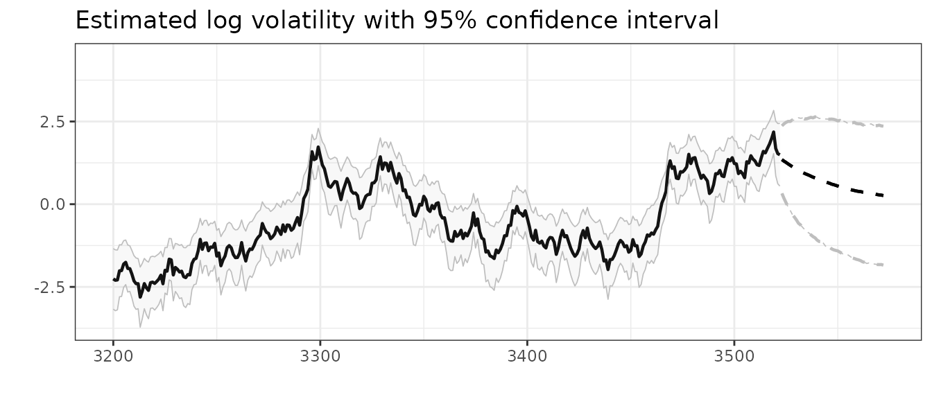

Checking the fit

plot_returns shows the returns together with the central 95% interval of the fitted conditional distribution of each return, given the estimated log-volatility. The interval uses the error distribution of the model, so it is asymmetric for the skew-Gaussian models. Returns outside the interval are red, and the subtitle gives their share. For a good model the share is close to 5%. The interval uses the smoothed log-volatility, which also uses the return on the same day, so this is an optimistic, in-sample check.

plot_returns(skew_t_leverage, dates = spy$date)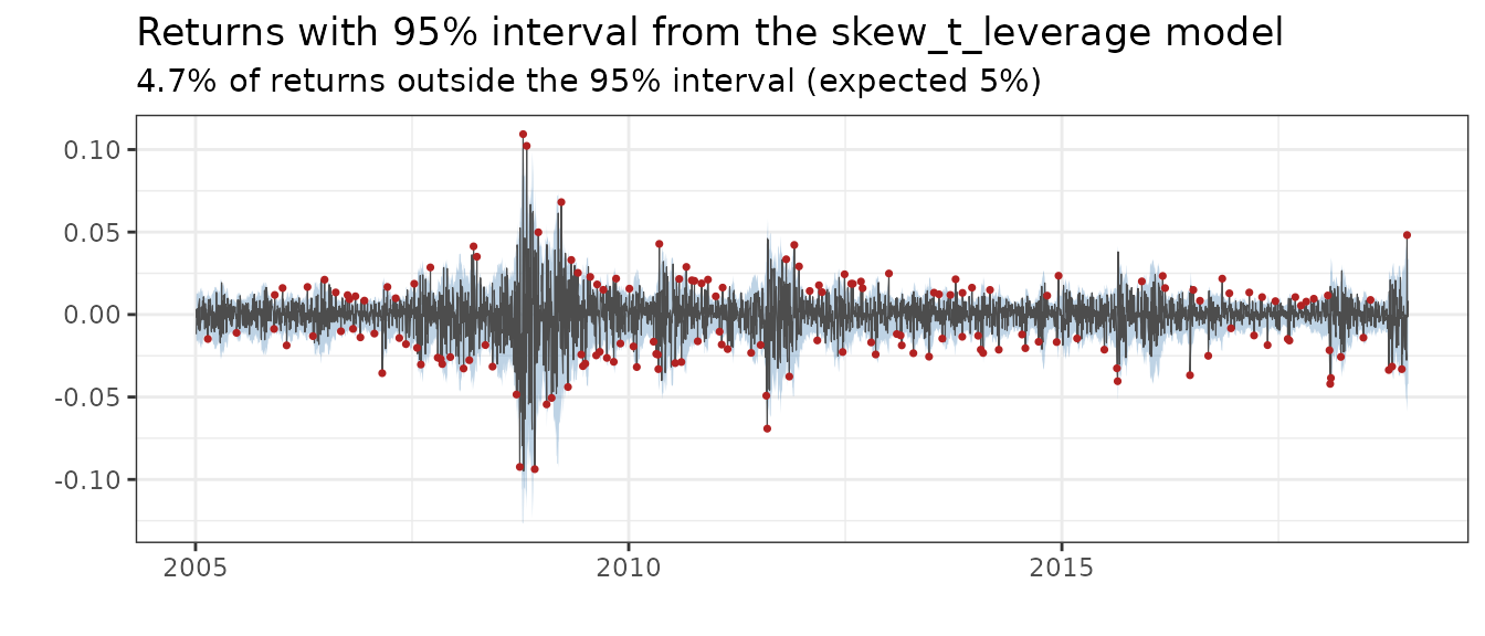

A stricter check uses one-step-ahead (OSA) residuals (Thygesen et al. (2017)). The OSA residual of \(y_t\) is \(\Phi^{-1}(F_t(y_t))\), where \(F_t\) is the predictive distribution function of \(y_t\) given \(y_1, \dots, y_{t-1}\). If the model is correct, the OSA residuals are independent and standard Gaussian. Because the log-volatility \(h_t\) is one-dimensional, residuals calculates \(F_t\) exactly with a filter on a grid for \(h_t\), for all observations in a few seconds (see One-step-ahead residuals for the details). The slower method based on the Laplace approximation, TMB::oneStepPredict, is available with method = "tmb".

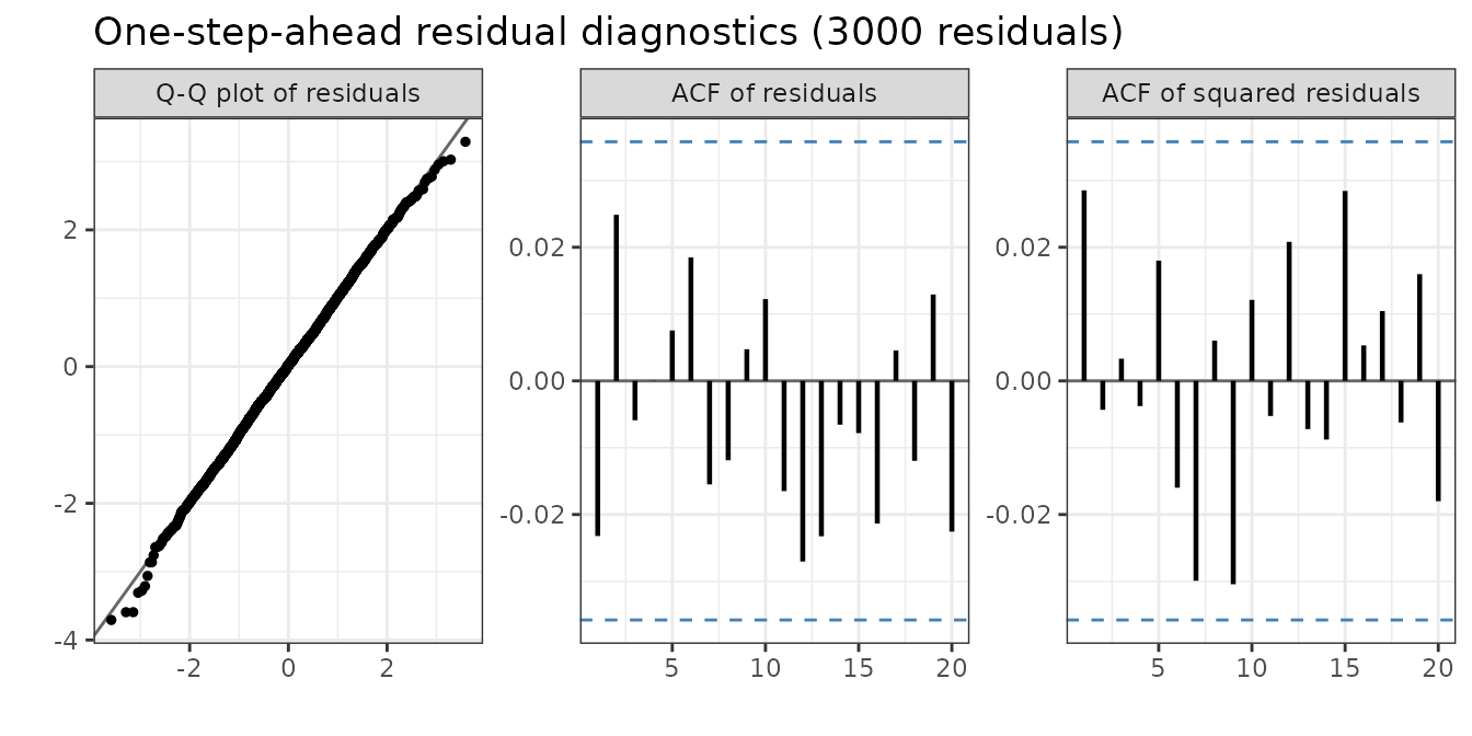
plot_diagnostics shows three panels:

• A Q-Q plot against the standard Gaussian distribution. Bent tails show that the error distribution is wrong.
• The autocorrelation function (ACF) of the residuals. Bars outside the dashed lines show dependence in the returns that the model does not capture.
• The ACF of the squared residuals. Bars outside the dashed lines show volatility clustering that the model does not capture.

We compare the Gaussian model with the skew-t model with leverage:

plot_diagnostics(gaussian)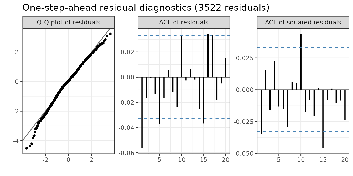

plot_diagnostics(skew_t_leverage)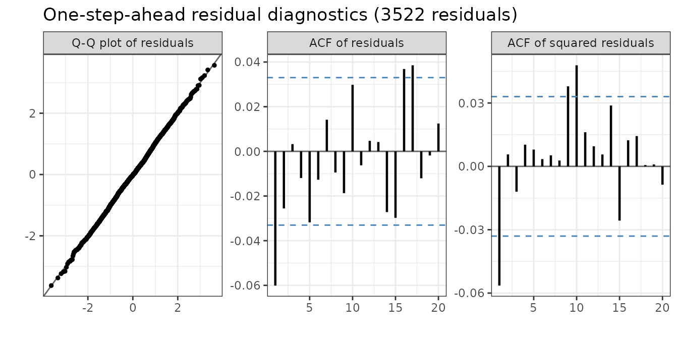

For the Gaussian model the Q-Q plot bends down in the left tail: there are more large negative returns than the model expects. For the skew-t model with leverage the Q-Q plot is a straight line, also for the most extreme negative returns. The heavy and asymmetric tails together with the leverage effect capture the distribution of the returns. Both models leave a small negative autocorrelation at lag 1 in the residuals. The models have mean zero and therefore cannot capture this. For the skew-t model with leverage, the autocorrelation of the squared residuals at lag 1 is also negative. This suggests that, after a large shock, the model increases the predicted volatility slightly too much.

Value at Risk and Expected Shortfall

A common use of a volatility model is to measure the risk of a position. For a level \(\alpha\), for example \(\alpha = 0.99\), the one-day Value at Risk (VaR) is the loss that the return on day \(t\) is below only with probability \(1 - \alpha\). The Expected Shortfall (ES) is the expected loss on the days when the loss is larger than the VaR. Let \(q_t\) be the \(1 - \alpha\) quantile of the predictive distribution \(F_t\) of \(y_t\) given \(y_1, \dots, y_{t-1}\). Then \[\begin{equation} \mathrm{VaR}_t = -q_t, \qquad \mathrm{ES}_t = -\mathrm{E}[y_t \mid y_t \le q_t, y_1, \dots, y_{t-1}]. \end{equation}\] Both are positive numbers when they are losses, on the scale of the log-returns.

var_es calculates \(F_t\) with the same filter as the one-step-ahead residuals (see One-step-ahead residuals). On the grid, \(F_t\) is a mixture: \(F_t(y) = \sum_j w_t(j) F(y \mid g_j)\). In all models, \(y_t / (\sigma_y e^{h_t/2})\) given \(h_t\) has a fixed standardized distribution \(G\) with mean zero and unit variance, so \(F(y \mid g_j) = G(y / s_j)\) with \(s_j = \sigma_y e^{g_j/2}\). The quantile \(q_t\) is the root of \(F_t(q) = 1 - \alpha\), and \[\begin{equation} \mathrm{ES}_t = -\frac{1}{1 - \alpha} \sum_j w_t(j) \, s_j \, M\left(\frac{q_t}{s_j}\right), \qquad M(c) = \mathrm{E}[Z \, 1(Z \le c)], \; Z \sim G. \end{equation}\] \(M\) has a closed form for the Gaussian, t and skew-Gaussian distributions. For the skew t distribution it is calculated numerically on a fine grid. var_es returns one row for each day and level, and the last row is the forecast for the next day after the data:

risk <- var_es(skew_t_leverage, level = c(0.95, 0.99))
risk[is.na(y)]
#>     time level     y        var         es exceedance
#>    <int> <num> <num>      <num>      <num>     <lgcl>
#> 1:  3523  0.95    NA 0.03181108 0.04560319         NA
#> 2:  3523  0.99    NA 0.05359064 0.06893175         NA

The parameters are fixed at their estimates from all the data, so the values for the observed days are in-sample.

Backtesting

A return is an exceedance if \(y_t < -\mathrm{VaR}_t\). For a correct model, the exceedances happen on a fraction \(1 - \alpha\) of the days, independently of each other. backtest_var tests both:

• The unconditional coverage test of Kupiec (1995) compares the number of exceedances with the expected number. A small p-value (p_uc) means that there are too many or too few exceedances.
• The independence test of Christoffersen (1998) checks if an exceedance is more likely on the day after an exceedance. A small p-value (p_ind) means that the exceedances come in clusters. This happens when the model reacts too slowly to a change in volatility.
• The conditional coverage test combines the two (p_cc).

es_ratio is the mean of \(-y_t / \mathrm{ES}_t\) over the exceedances. It is close to one when the ES is correct.

backtest_var(risk)
#>    level     n expected observed        rate      lr_uc      p_uc    lr_ind
#>    <num> <int>    <num>    <int>       <num>      <num>     <num>     <num>
#> 1:  0.95  3522   176.10      191 0.054230551 1.29303116 0.2554901 1.3599331
#> 2:  0.99  3522    35.22       34 0.009653606 0.04318348 0.8353802 0.9112984
#>        p_ind     lr_cc      p_cc  es_ratio
#>        <num>     <num>     <num>     <num>
#> 1: 0.2435491 2.6529642 0.2654093 0.9890637
#> 2: 0.3397702 0.9544819 0.6204930 1.0067746
backtest_var(var_es(gaussian, level = c(0.95, 0.99)))
#>    level     n expected observed       rate    lr_uc         p_uc   lr_ind
#>    <num> <int>    <num>    <int>      <num>    <num>        <num>    <num>
#> 1:  0.95  3522   176.10      208 0.05905735  5.76331 0.0163642133 1.083807
#> 2:  0.99  3522    35.22       60 0.01703578 14.54418 0.0001369108 2.638690
#>        p_ind     lr_cc         p_cc es_ratio
#>        <num>     <num>        <num>    <num>
#> 1: 0.2978474  6.847118 0.0325962219 1.094632
#> 2: 0.1042895 17.182871 0.0001856893 1.080347

The Gaussian model has too many exceedances, in particular at the 99% level, because its tails are too light. The skew-t model with leverage has close to the expected number of exceedances at both levels, and its es_ratio is close to one. plot_var shows the returns with \(-\mathrm{VaR}_t\) and \(-\mathrm{ES}_t\) and marks the exceedances:

plot_var(risk, level = 0.99, dates = spy$date)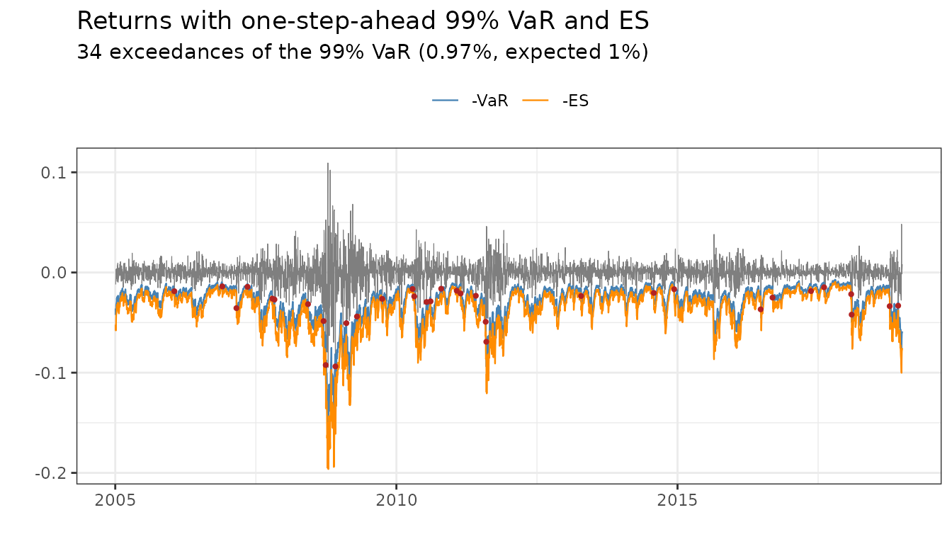

More than one day ahead

For more than one day there is no simple formula for the distribution of the returns. forecast_var_es therefore simulates future paths with predict and calculates VaR and ES for each day ahead, both for the return on that day and for the cumulative return up to that day. By default, the simulation includes the uncertainty of the parameters. predict starts from a Gaussian approximation of the last log-volatility, so for one day ahead the result differs slightly from the exact var_es:

set.seed(1)
forecast_var_es(skew_t_leverage, steps = 10, level = 0.99)
#>      step level        var         es var_cumulative es_cumulative
#>     <int> <num>      <num>      <num>          <num>         <num>
#>  1:     1  0.99 0.05321239 0.06872867     0.05321239    0.06872867
#>  2:     2  0.99 0.05466494 0.07102813     0.07654920    0.09854347
#>  3:     3  0.99 0.05392145 0.07070557     0.09661490    0.12275207
#>  4:     4  0.99 0.05404943 0.07126835     0.11197686    0.14337785
#>  5:     5  0.99 0.05398812 0.07171376     0.12566563    0.16325650
#>  6:     6  0.99 0.05388871 0.07200359     0.13942413    0.17975980
#>  7:     7  0.99 0.05431752 0.07300936     0.15104218    0.19599194
#>  8:     8  0.99 0.05406979 0.07313807     0.16243718    0.21102743
#>  9:     9  0.99 0.05427650 0.07360896     0.17503939    0.22806235
#> 10:    10  0.99 0.05287490 0.07258450     0.18626579    0.24215530

Comparison to stochvol

The R-package stochvol (Kastner (2016)) provides a Bayesian framework for inference using Markov Chain Monte Carlo. An advantage of stochvolTMB is that optimization can be a lot faster than MCMC. We here compare the leverage and the gaussian model. Depending on your machine you can expect a speed up of 20-200x.

library(stochvol)

stochvol_gauss <- svsample(spy$log_return, quiet = T)
stochvolTMB_gauss  <- estimate_parameters(spy$log_return, "gaussian", silent = TRUE)

stochvol_lev <- svlsample(spy$log_return, quiet = T)
stochvolTMB_lev  <- estimate_parameters(spy$log_return, "leverage", silent = TRUE)

We can compare the parameter estimates of the two methods. Note that the parameter exp(mu/2) and sigma from stochvol is the same as sigma_y and sigma_h from stochvolTMB. Both methods give almost identical results.

stochvol_gauss$para
#>                   mean           sd          5%          50%          95%
#> mu        -9.611533785 0.1854455626 -9.91175182 -9.611774497 -9.304678419
#> phi        0.978189757 0.0049148914  0.96968612  0.978414831  0.985836137
#> sigma      0.229775055 0.0203786934  0.19733459  0.228942708  0.264098047
#> exp(mu/2)  0.008217761 0.0007671236  0.00704191  0.008181439  0.009539261
#> sigma^2    0.053211825 0.0094502446  0.03894094  0.052414764  0.069747778
#>                 ESS
#> mu        6230.1953
#> phi        327.9347
#> sigma      152.4001
#> exp(mu/2) 6230.1953
#> sigma^2    152.4001
summary(stochvolTMB_gauss, report = "transformed")
#>    parameter    estimate    std_error   z_value      p_value        type
#>       <char>       <num>        <num>     <num>        <num>      <char>
#> 1:   sigma_y 0.008185162 0.0007314791  11.18988 4.570586e-29 transformed
#> 2:   sigma_h 0.222440223 0.0190056672  11.70389 1.217431e-31 transformed
#> 3:       phi 0.979034243 0.0046595769 210.11226 0.000000e+00 transformed
stochvol_lev$para
#>                   mean           sd           5%          50%          95%
#> mu        -9.569375399 0.1053851888 -9.739817718 -9.571446103 -9.400002030
#> phi        0.966952934 0.0041187166  0.960195391  0.966853189  0.973557574
#> sigma      0.276351629 0.0172514582  0.248100974  0.277044222  0.304057250
#> rho       -0.724949416 0.0328632332 -0.775144574 -0.726905055 -0.667578807
#> exp(mu/2)  0.008368349 0.0004417329  0.007674065  0.008348085  0.009095268
#> sigma^2    0.076667806 0.0095068932  0.061554093  0.076753501  0.092450811
#>                 ESS
#> mu        368.69311
#> phi       140.52279
#> sigma      42.20112
#> rho        26.56514
#> exp(mu/2) 368.69311
#> sigma^2    42.20112
summary(stochvolTMB_lev, report = "transformed")
#>    parameter     estimate    std_error   z_value       p_value        type
#>       <char>        <num>        <num>     <num>         <num>      <char>
#> 1:   sigma_y  0.008338412 0.0004163314  20.02830  3.121144e-89 transformed
#> 2:   sigma_h  0.273443559 0.0182641070  14.97164  1.125191e-50 transformed
#> 3:       phi  0.967721215 0.0043681868 221.53842  0.000000e+00 transformed
#> 4:       rho -0.748695259 0.0322487815 -23.21623 3.121690e-119 transformed

Estimation

The R-package TMB (Kristensen et al. (2016)) is used to implement our models for maximum likelihood estimation, since TMB lets us estimate parameters in models with a high number of latent variables.

Parameter estimation of stochastic volatility models is hard due to the fact the likelihood function is expressed as a high dimensional integral over the latent variables that cannot be evaluated analytically. If \(\mathbf{y} = (y_1, \ldots, y_T)\) denotes our observations, \(\mathbf{h} = (h_1, \ldots, h_T)\) our latent variables and \(\mathbf{\theta}\) the parameters of interest, the likelihood of \(\mathbf{\theta}\) is given by

\[\begin{equation} \mathcal{L}(\mathbf{\theta}) = \int f_{\mathbf{y}}(\mathbf{y}|\mathbf{h})f_{\mathbf{h}}(\mathbf{h}) \, d\mathbf{h}, \end{equation}\]

The conditional density of our observations given \(\mathbf{h}\) is denoted by \(f_{\mathbf{y}}(\mathbf{y}|\mathbf{h})\), and \(f_{\mathbf{h}}(\mathbf{h})\) denotes the marginal density of \(\mathbf{h}\). To approximate this integral we apply the Laplace approximation.

Laplace Approximation

Let \(\mathbf{y}\) be a vector of observations, \(\mathbf{\theta}\) our parameters of interest and \(\mathbf{h}\) be a random vector of latent variables. Let \(g(\mathbf{h},\mathbf{\theta})\) denote the negative joint log-likelihood. The likelihood of \(\mathbf{\theta}\) is given by

\[\begin{equation} \mathcal{L}(\mathbf{\theta}) = \int f(\mathbf{y},\mathbf{h}) \, d\mathbf{h} = \int f_{\mathbf{y}}(\mathbf{y}|\mathbf{h}) f_{\mathbf{h}}(\mathbf{h}) \, d\mathbf{h} = \int \exp \{-g(\mathbf{h},\mathbf{\theta})\} \, d\mathbf{h}. \end{equation}\]

We assume that \(g\) has a global minimum at \(\mathbf{\hat{h}}\) for a given \(\mathbf{\theta}\), i.e. \(\mathbf{\hat{h}} = \text{argmin}_{\mathbf{h}} g(\mathbf{h},\mathbf{\theta})\), and that \(g\) is twice differentiable. The solution \(\hat{\mathbf{h}}\) is known as the Empirical Bayes (EB) estimate. A second order Taylor expansion around \(\mathbf{\hat{h}}\) yields

\[\begin{equation} g(\mathbf{h},\mathbf{\theta}) \approx g(\mathbf{\hat{h}},\mathbf{\theta}) + \nabla g(\mathbf{\hat{h}},\mathbf{\theta})(\mathbf{h} - \mathbf{\hat{h}}) + \frac{1}{2}(\mathbf{h} - \mathbf{\hat{h}})^T\mathbb{H}(\mathbf{h} - \mathbf{\hat{h}}) \end{equation}\]

Since \(\mathbf{\hat{h}}\) is a minimum, \(\nabla g(\mathbf{\hat{h}},\mathbf{\theta}) = 0\). Therefore

\[\begin{equation} \mathcal{L}(\mathbf{\theta}) \approx \exp \{-g(\mathbf{\hat{h}},\mathbf{\theta})\} \int \exp \bigg \{-\frac{1}{2}(\mathbf{h} - \mathbf{\hat{h}})^T\mathbb{H}(\mathbf{h} - \mathbf{\hat{h}}) \bigg \} d\mathbf{h} \end{equation}\]

We can observe that the integrand is the kernel of a multivariate normal density with covariance matrix \(\mathbb{H}^{-1}\). The approximation is therefore given by

\[\begin{equation} \mathcal{L}(\mathbf{\theta}) \approx \exp \{-g(\mathbf{\hat{h}},\mathbf{\theta})\} (2\pi)^{\text{dim}(\mathbf{h})/2} \text{det}(\mathbb{H})^{-1/2}, \end{equation}\]

where we have used the fact that \(\text{det}(\mathbb{H}^{-1}) = \text{det}(\mathbb{H})^{-1}\). The corresponding negative log-likelihood is

\[\begin{equation} -l(\mathbf{\theta}) = -\frac{\text{dim}(\mathbf{h})}{2} \log (2\pi) + \frac{1}{2} \log \text{det}(\mathbb{H}) + g(\mathbf{\hat{h}},\mathbf{\theta}). \end{equation}\]

Finding the optimal value of \(\mathbf{\theta}\) can be viewed as a nested optimization problem. To find \(\mathbf{h} (\mathbf{\theta})\) and \(\mathbb{H}(\mathbf{\theta})\) we fix \(\mathbf{\theta}\) and optimize using a quasi-Newton algorithm or a limited memory Newton method. The Laplace approximation is then optimized w.r.t. \(\mathbf{\theta}\) using the quasi-Newton algorithm.

One-step-ahead residuals

This section explains how residuals calculates the one-step-ahead (OSA) residuals that plot_diagnostics uses. The parameters \(\mathbf{\theta}\) are fixed at their estimates, so we do not write them below.

Why OSA residuals are standard Gaussian

Let \(F_t(y) = P(y_t \le y \mid y_1, \dots, y_{t-1})\) be the distribution function of \(y_t\) given the earlier observations. This is the predictive distribution of \(y_t\): what the model expects for day \(t\), given everything until day \(t-1\). The OSA residual of \(y_t\) is \[\begin{equation} r_t = \Phi^{-1}\big(F_t(y_t)\big), \end{equation}\] where \(\Phi^{-1}\) is the quantile function of the standard Gaussian distribution.

If the model is correct, \(u_t = F_t(y_t)\) is uniform on \((0, 1)\). This is the probability integral transform: if a random variable \(Y\) has a continuous distribution function \(F\), then \(F(Y)\) is uniform. Because \(\Phi^{-1}\) maps a uniform variable to a standard Gaussian variable, \(r_t\) is standard Gaussian. Each \(u_t\) is calculated given the earlier observations only, so \(u_1, \dots, u_T\) are also independent (Thygesen et al. (2017)). In summary, for a correct model the OSA residuals are independent and standard Gaussian.

A large negative residual means that the model gave a very small probability to a return that low, given the earlier returns. That is why the Q-Q plot of the OSA residuals shows if the tails of the model are correct.

Note that ordinary residuals, for example \(y_t / (\sigma_y e^{\hat{h}_t/2})\) with the estimated \(\hat{h}_t\), do not have this property. The estimate \(\hat{h}_t\) uses all observations, also \(y_t\) itself and the observations after \(t\).

The filter

The difficulty is that \(F_t\) depends on the unobserved log-volatility \(h_t\). Given \(h_t\), the distribution of \(y_t\) is known, for example \(y_t \mid h_t \sim \mathcal{N}(0, \sigma_y^2 e^{h_t})\) in the Gaussian model. We write \(F(y \mid h_t)\) for this conditional distribution function and \(f(y \mid h_t)\) for its density. But \(h_t\) is not known, only its distribution given the earlier observations. We call this the predictive density of \(h_t\): \[\begin{equation} \pi_t(h) = p(h_t = h \mid y_1, \dots, y_{t-1}). \end{equation}\] Then \(F_t\) is the average of \(F(y \mid h)\) over this density: \[\begin{equation} F_t(y) = \int F(y \mid h) \, \pi_t(h) \, dh. \end{equation}\]

We calculate \(\pi_t\) for \(t = 1, \dots, T\) with a filter. A filter goes once forward through the data and repeats three steps for each day:

1. Predict. Use \(\pi_t\) to calculate \(F_t(y_t)\) and the residual \(r_t\).
2. Update. Use Bayes’ rule to include \(y_t\). The density of \(h_t\) given \(y_1, \dots, y_t\) is \[\begin{equation} p(h_t = h \mid y_1, \dots, y_t) = \frac{f(y_t \mid h) \, \pi_t(h)}{\int f(y_t \mid h') \, \pi_t(h') \, dh'}. \end{equation}\]
3. Move forward. Use the model for \(h_{t+1}\) given \(h_t\), which is \(\mathcal{N}(\phi h_t, \sigma_h^2)\), to get the predictive density for the next day: \[\begin{equation} \pi_{t+1}(h') = \int \frac{1}{\sigma_h} \varphi\left(\frac{h' - \phi h}{\sigma_h}\right) p(h_t = h \mid y_1, \dots, y_t) \, dh, \end{equation}\] where \(\varphi\) is the standard Gaussian density.

The filter starts with the stationary distribution, \(\pi_1 = \mathcal{N}(0, \sigma_h^2 / (1 - \phi^2))\).

From integrals to sums

The integrals above have no closed form. But \(h_t\) is one-dimensional, so we can calculate them accurately on a grid. Let \(g_1 < g_2 < \dots < g_G\) be \(G\) equally spaced points that cover eight stationary standard deviations of \(h_t\) on each side of zero. By default \(G = 500\). We keep \(\pi_t\) as a vector of weights \(w_t(j) \approx \pi_t(g_j) \Delta\), where \(\Delta\) is the distance between the grid points, and the weights sum to one. The three steps become sums: \[\begin{equation} \begin{aligned} F_t(y_t) &= \sum_{j=1}^G w_t(j) \, F(y_t \mid g_j), \\ \tilde{w}_t(j) &= \frac{f(y_t \mid g_j) \, w_t(j)}{\sum_{i=1}^G f(y_t \mid g_i) \, w_t(i)}, \\ w_{t+1}(k) &= \sum_{j=1}^G \tilde{w}_t(j) \, P_{jk}. \end{aligned} \end{equation}\] Here \(P_{jk}\) is the probability of moving from \(g_j\) to \(g_k\). It is proportional to \(\varphi\big((g_k - \phi g_j) / \sigma_h\big)\), scaled so that each row of \(P\) sums to one.

The only error is from the grid. With 500 grid points, the residuals for the S&P 500 data change by less than \(10^{-7}\) when we use 1000 grid points instead. Most grid points have a weight that is almost zero, so the sums skip the points with a weight below \(10^{-14}\) times the largest weight. This makes the filter fast: one pass over 3522 observations takes a few seconds.

Models with leverage

In the leverage models, \(y_t\) and \(h_{t+1}\) are correlated. The filter then needs one more step.

In the skew-Gaussian and the skew-t model with leverage, \(y_t\) depends on \(h_t\) only, so steps 1 and 2 do not change. The return shock \(z_t = y_t / (\sigma_y e^{h_t/2})\) drives the next volatility shock, so in step 3 the model for \(h_{t+1}\) also depends on \(y_t\): \[\begin{equation} h_{t+1} \mid h_t, y_t \sim \mathcal{N}\left(\phi h_t + \sigma_h \rho z_t, \; \sigma_h^2 (1 - \rho^2)\right). \end{equation}\] The transition probabilities \(P_{jk}\) therefore change from day to day. They are proportional to \(\varphi\big((g_k - \phi g_j - \sigma_h \rho z_{t,j}) / (\sigma_h \sqrt{1 - \rho^2})\big)\), where \(z_{t,j} = y_t / (\sigma_y e^{g_j/2})\).

In the Gaussian model with leverage, \(y_t\) depends on both \(h_t\) and \(h_{t+1}\), through the volatility shock \(\eta_t = (h_{t+1} - \phi h_t) / \sigma_h\): \[\begin{equation} y_t \mid h_t, h_{t+1} \sim \mathcal{N}\left(\sigma_y e^{h_t/2} \rho \eta_t, \; \sigma_y^2 e^{h_t} (1 - \rho^2)\right). \end{equation}\] The filter therefore works with the joint predictive weights of \((h_t, h_{t+1})\) on the grid, \(w_t(j) P_{jk}\). Steps 1 and 2 sum over both \(j\) and \(k\), and the sum over \(j\) gives the weights for \(h_{t+1}\). Step 1 can also use that \(y_t \mid h_t \sim \mathcal{N}(0, \sigma_y^2 e^{h_t})\) once \(h_{t+1}\) is integrated out.

Comparison with the Laplace approximation

TMB::oneStepPredict, which is available with residuals(method = "tmb"), calculates the same residuals in a different way. For each observation it integrates over \(y_t\) numerically, and each point of that integral needs a full Laplace approximation over all \(T\) latent variables. It is not available for the skew-t model with leverage, because there \(y_t\) also enters the model for \(h_{t+1}\), which oneStepPredict does not allow. This takes one to three seconds per observation, and the Laplace approximation can be inaccurate in the tails. The grid filter uses that \(h_t\) is one-dimensional and that the model is a Markov chain in \(h_t\). It therefore needs only one pass over the data and does not use the Laplace approximation.

We can check the method on simulated data. If we simulate from a model and fit the same model, the OSA residuals must be standard Gaussian and independent:

param <- list(phi = 0.95, sigma_h = 0.3, sigma_y = 0.01, alpha = -3, rho = -0.7)
sim <- sim_sv(param, nobs = 3000, seed = 2, model = "skew_gaussian_leverage")
fit_sim <- estimate_parameters(sim$y, model = "skew_gaussian_leverage", silent = TRUE)
plot_diagnostics(fit_sim)

References

Christoffersen, Peter F. 1998. “Evaluating Interval Forecasts.” International Economic Review 39 (4): 841–62. https://doi.org/10.2307/2527341.

Jones, M. C., and M. J. Faddy. 2003. “A Skew Extension of the t-Distribution, with Applications.” Journal of the Royal Statistical Society: Series B (Statistical Methodology) 65 (1): 159–74. https://doi.org/10.1111/1467-9868.00378.

Kastner, Gregor. 2016. “Dealing with Stochastic Volatility in Time Series Using the R Package stochvol.” Journal of Statistical Software 69 (5): 1–30. https://doi.org/10.18637/jss.v069.i05.

Kristensen, Kasper, Anders Nielsen, Casper Berg, Hans Skaug, and Bradley Bell. 2016. “TMB: Automatic Differentiation and Laplace Approximation.” Journal of Statistical Software, Articles 70 (5): 1–21. https://doi.org/10.18637/jss.v070.i05.

Kupiec, Paul H. 1995. “Techniques for Verifying the Accuracy of Risk Measurement Models.” The Journal of Derivatives 3 (2): 73–84. https://doi.org/10.3905/jod.1995.407942.

Taylor, S. J. 1982. “Financial Returns Modelled by the Product of Two Stochastic Processes-a Study of the Daily Sugar Prices 1961-75.” Time Series Analysis : Theory and Practice 1: 203–26.

Thygesen, Uffe Høgsbro, Christoffer Moesgaard Albertsen, Casper W. Berg, Kasper Kristensen, and Anders Nielsen. 2017. “Validation of Ecological State Space Models Using the Laplace Approximation.” Environmental and Ecological Statistics 24 (2): 317–39. https://doi.org/10.1007/s10651-017-0372-4.